Convolution and deconvolution: an Illustration
This Jupyter notebook in a Quarto slideshow is translated from a Matlab LiveScript. The code visualizes some of the elements of convolution and deconvolution
- Convolution: a simple mathematical function that quantifies similarity between a pattern (a “kernel”) such as the red square wave below with data ( blue rectangularish thingy below).
The convolution (black line) reflects how similar the blue signal is with the kernel at any given time point. Convolution is thus used in all of digital signal processing.
Convolution in signal generation and in fMRI research.
if we want to generate a signal where a certain pattern (the kernel) occurs at certain times, we can use convolution to achieve that. Thus, programs liek SPM use convolution of stimulus timinng info with a lernel that resembles the typical BOLD (fMRI) response as the kernel to generate fake, ideal, fMRI activation for comparison/correlation with the real data:
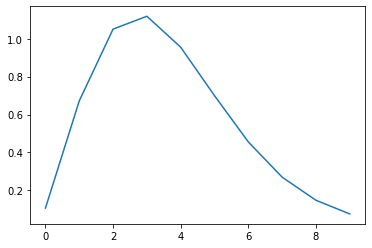
Make a Kernel
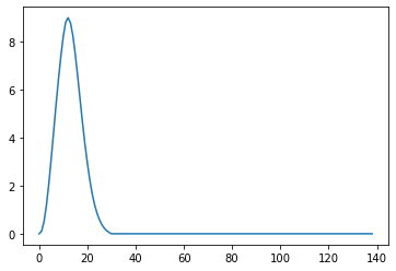
- Now we make a kernel.
- the inverted gamma function is nice because it looks like fMRI in V1
- let’s make one that is 10 scans long
convolve
Now we just convolve the onsets with the kernel and plot the result

longer onsets
So this basically puts each 10 second kernel at the location where the onset is. There were 11 seconds between onsets, so this is like copy paste, but how about when the kernel is longer than the interval between onsets?

but
So this basically puts each 10 second kernel at the location where the onset is. There were 11 seconds between onsets, so this is like copy paste, but how about when the kernel is longer than the interval between onsets?
even better…
This is more interesting with variable inter-onset times.

Now we convolve these onset times with the same kernel
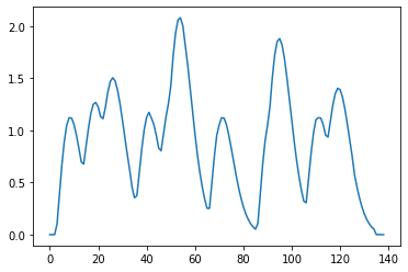
what happened?
Longer intervals between onsets prompt complete reduction to baseline, temporal proximity prompts smeared, overlapping events. How about gamma-shaped responses to stimuli that are longer than one image?
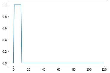
onsets = np.zeros((120,1))
set0=[3,14,22,36,46,50,66,86,91,106,115];
set1=[i+1 for i in set0]
set2=[i+2 for i in set0]
set3=[i+3 for i in set0]
onsets[set0,] = 1; #simple case where a stimulus is on every 11 scans
onsets[set1,] = 1;

onsets[set2,] = 1;#simple case where a stimulus is on every 11 scans
onsets[set3,] = 1;
##onsets[[3, 14, 22, 36, 46, 50, 66, 86, 91, 106, 115]+2,] = 1;
#onsets[[3, 14, 22, 36, 46, 50, 66, 86, 91, 106, 115]+3,] = 1;
plt.plot(onsets) #, title ('simulated stimulus onsets, every 11 scans')
next
Now we convolve these onset times with the same kernel

Deconvolution
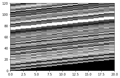
deconvolution is the process where we wish to estimate the Kernel from known data and known event-times. This is a version of the so-called inverse problem , and we solve it with a regression. Let’s start with the simulated we we have:
convolution = np.random.rand(200) # Replace with your own convolution array
onsets = np.random.rand(120) # Replace with your own onsets array

X = np.zeros((len(convolution[0:120]), 20))
temp = onsets.copy()

for i in range(20):
    X[:, i] = temp
    temp = np.concatenate(([0], temp[:-1]))

plt.pcolor(X, cmap='gray')
plt.show()